Simple Binary Classification with Sigmoid Activation#
Packages#
import numpy as np
import matplotlib.pyplot as plt
from matplotlib import colors
# A function to create a dataset.
from sklearn.datasets import make_blobs

# Output of plotting commands is displayed inline within the Jupyter notebook.
%matplotlib inline

# Set a seed so that the results are consistent.
np.random.seed(3)
1 - Single Perceptron Neural Network with Activation Function#
You already have constructed and trained a neural network model with one perceptron. Here a similar model can be used, but with an activation function. Then a single perceptron basically works as a threshold function.
1.1 - Neural Network Structure#
The neural network components are shown in the following scheme:
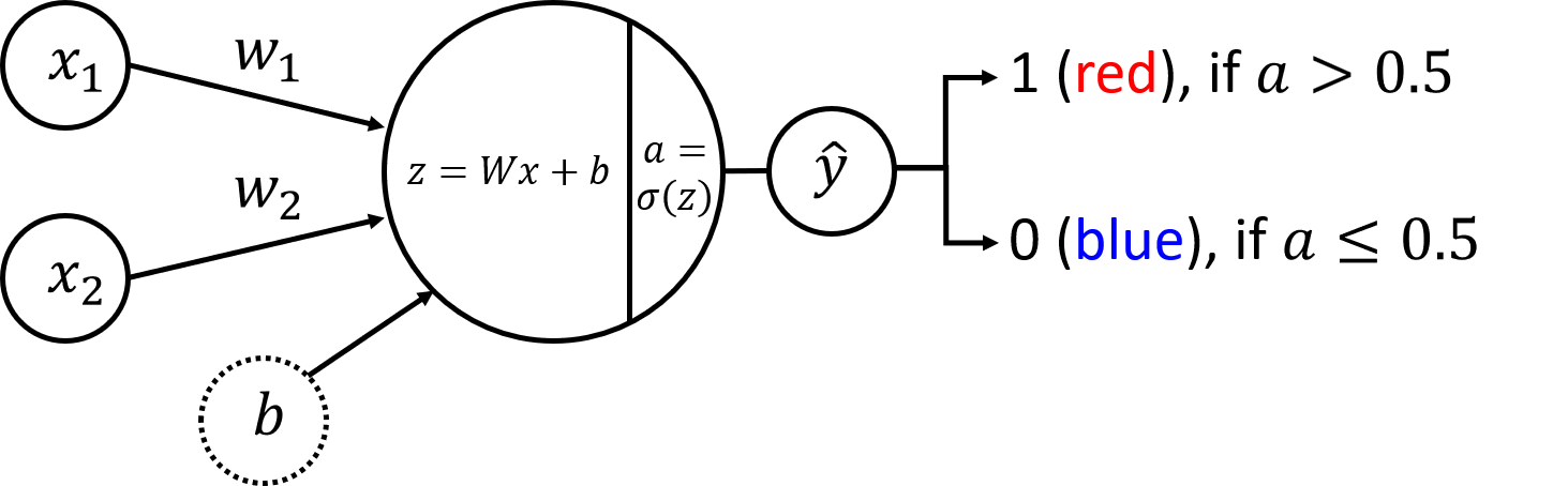
Neural Network Structure#
Similarly to the previous lab, the input layer contains two nodes \(x_1\) and \(x_2\). Weight vector \(W = \begin{bmatrix} w_1 & w_2\end{bmatrix}\) and bias (\(b\)) are the parameters to be updated during the model training. First step in the forward propagation is the same as in the previous lab. For every training example \(x^{(i)} = \begin{bmatrix} x_1^{(i)} & x_2^{(i)}\end{bmatrix}\):
But now you cannot take a real number \(z^{(i)}\) into the output as you need to perform classification. It could be done with a discrete approach: compare the result with zero, and classify as \(0\) (blue) if it is below zero and \(1\) (red) if it is above zero. Then define cost function as a percentage of incorrectly identified classes and perform backward propagation.
This extra step in the forward propagation is actually an application of an activation function. It would be possible to implement the discrete approach described above (with unit step function) for this problem, but it turns out that there is a continuous approach that works better and is commonly used in more complicated neural networks. So you will implement it here: single perceptron with sigmoid activation function.
Sigmoid activation function is defined as
Then a threshold value of \(0.5\) can be used for predictions: \(1\) (red) if \(a > 0.5\) and \(0\) (blue) otherwise. Putting it all together, mathematically the single perceptron neural network with sigmoid activation function can be expressed as:
If you have \(m\) training examples organised in the columns of (\(2 \times m\)) matrix \(X\), you can apply the activation function element-wise. So the model can be written as:
where \(b\) is broadcasted to the vector of a size (\(1 \times m\)).
When dealing with classification problems, the most commonly used cost function is the log loss, which is described by the following equation:
where \(y^{(i)} \in \{0,1\}\) are the original labels and \(a^{(i)}\) are the continuous output values of the forward propagation step (elements of array \(A\)).
You want to minimize the cost function during the training. To implement gradient descent, calculate partial derivatives using chain rule:
As discussed in the videos, \(\frac{\partial L }{ \partial a^{(i)}} \frac{\partial a^{(i)} }{ \partial z^{(i)}} = \left(a^{(i)} - y^{(i)}\right)\), \(\frac{\partial z^{(i)}}{ \partial w_1} = x_1^{(i)}\), \(\frac{\partial z^{(i)}}{ \partial w_2} = x_2^{(i)}\) and \(\frac{\partial z^{(i)}}{ \partial b} = 1\). Then \((6)\) can be rewritten as:
Note that the obtained expressions \((7)\) are exactly the same as in the section \(3.2\) of the previous lab, when multiple linear regression model was discussed. Thus, they can be rewritten in a matrix form:
where \(\left(A - Y\right)\) is an array of a shape (\(1 \times m\)), \(X^T\) is an array of a shape (\(m \times 2\)) and \(\mathbf{1}\) is just a (\(m \times 1\)) vector of ones.
Then you can update the parameters:
where \(\alpha\) is the learning rate. Repeat the process in a loop until the cost function stops decreasing.
Finally, the predictions for some example \(x\) can be made taking the output \(a\) and calculating \(\hat{y}\) as
- Dataset#
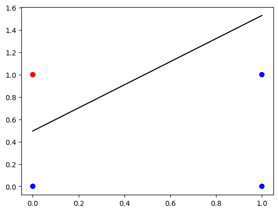
Let’s get the dataset you will work on. The following code will create \(m=30\) data points \((x_1, x_2)\), where \(x_1, x_2 \in \{0,1\}\) and save them in the NumPy array X of a shape \((2 \times m)\) (in the columns of the array). The labels (\(0\): blue, \(1\): red) will be calculated so that \(y = 1\) if \(x_1 = 0\) and \(x_2 = 1\), in the rest of the cases \(y=0\). The labels will be saved in the array Y of a shape \((1 \times m)\).
m = 30

X = np.random.randint(0, 2, (2, m))
Y = np.logical_and(X[0] == 0, X[1] == 1).astype(int).reshape((1, m))

print('Training dataset X containing (x1, x2) coordinates in the columns:')
print(X)
print('Training dataset Y containing labels of two classes (0: blue, 1: red)')
print(Y)

print ('The shape of X is: ' + str(X.shape))
print ('The shape of Y is: ' + str(Y.shape))
print ('I have m = %d training examples!' % (X.shape[1]))
- Define Activation Function#
The sigmoid function \((2)\) for a variable \(z\) can be defined with the following code:
def sigmoid(z):
    return 1/(1 + np.exp(-z))

print("sigmoid(-2) = " + str(sigmoid(-2)))
print("sigmoid(0) = " + str(sigmoid(0)))
print("sigmoid(3.5) = " + str(sigmoid(3.5)))
It can be applied to a NumPy array element by element:
print(sigmoid(np.array([-2, 0, 3.5])))
2 - Implementation of the Neural Network Model#
Implementation of the described neural network will be very similar to the regression_with_single_perceptron lab. The differences will be only in the functions forward_propagation and compute_cost!
def layer_sizes(X, Y):
    """
    Arguments:
    X -- input dataset of shape (input size, number of examples)
    Y -- labels of shape (output size, number of examples)

    Returns:
    n_x -- the size of the input layer
    n_y -- the size of the output layer
    """
    n_x = X.shape[0]
    n_y = Y.shape[0]

    return (n_x, n_y)

(n_x, n_y) = layer_sizes(X, Y)
print("The size of the input layer is: n_x = " + str(n_x))
print("The size of the output layer is: n_y = " + str(n_y))
def initialize_parameters(n_x, n_y):
    """
    Returns:
    params -- python dictionary containing your parameters:
                    W -- weight matrix of shape (n_y, n_x)
                    b -- bias value set as a vector of shape (n_y, 1)
    """

    W = np.random.randn(n_y, n_x) * 0.01
    b = np.zeros((n_y, 1))

    parameters = {"W": W,
                  "b": b}

    return parameters

parameters = initialize_parameters(n_x, n_y)
print("W = " + str(parameters["W"]))
print("b = " + str(parameters["b"]))
Implement forward_propagation() following the equation \((4)\):
$\(
Z = W X + b
\)\(
\)\(
A = \sigma\left(Z\right).
\)$
def forward_propagation(X, parameters):
    """
    Argument:
    X -- input data of size (n_x, m)
    parameters -- python dictionary containing your parameters (output of initialization function)

    Returns:
    A -- The output
    """
    W = parameters["W"]
    b = parameters["b"]

    # Forward Propagation to calculate Z.
    Z = W @ X + b
    A = sigmoid(Z)

    return A

A = forward_propagation(X, parameters)

print("Output vector A:", A)
Your weights were just initialized with some random values, so the model has not been trained yet.
Define a cost function \((5)\) which will be used to train the model:
def compute_cost(A, Y):
    """
    Computes the log loss cost function

    Arguments:
    A -- The output of the neural network of shape (n_y, number of examples)
    Y -- "true" labels vector of shape (n_y, number of examples)

    Returns:
    cost -- log loss

    """
    # Number of examples.
    m = Y.shape[1]

    # Compute the cost function.
    logprobs = - (Y * np.log(A)) - (1 - Y) * np.log(1 - A)
    cost = 1/m * np.sum(logprobs)

    return cost

print("cost = " + str(compute_cost(A, Y)))
Calculate partial derivatives as shown in \((8)\):
def backward_propagation(A, X, Y):
    """
    Implements the backward propagation, calculating gradients

    Arguments:
    A -- the output of the neural network of shape (n_y, number of examples)
    X -- input data of shape (n_x, number of examples)
    Y -- "true" labels vector of shape (n_y, number of examples)

    Returns:
    grads -- python dictionary containing gradients with respect to different parameters
    """
    m = X.shape[1]

    # Backward propagation: calculate partial derivatives denoted as dW, db for simplicity.
    dZ = A - Y
    dW = 1/m * (dZ @ X.T)
    db = 1/m * np.sum(dZ, axis = 1, keepdims = True)

    grads = {"dW": dW,
             "db": db}

    return grads

grads = backward_propagation(A, X, Y)

print("dW = " + str(grads["dW"]))
print("db = " + str(grads["db"]))
Update parameters as shown in \((9)\):
def update_parameters(parameters, grads, learning_rate=1.2):
    """
    Updates parameters using the gradient descent update rule

    Arguments:
    parameters -- python dictionary containing parameters
    grads -- python dictionary containing gradients
    learning_rate -- learning rate parameter for gradient descent

    Returns:
    parameters -- python dictionary containing updated parameters
    """
    # Retrieve each parameter from the dictionary "parameters".
    W = parameters["W"]
    b = parameters["b"]

    # Retrieve each gradient from the dictionary "grads".
    dW = grads["dW"]
    db = grads["db"]

    # Update rule for each parameter.
    W = W - learning_rate * dW
    b = b - learning_rate * db

    parameters = {"W": W,
                  "b": b}

    return parameters

parameters_updated = update_parameters(parameters, grads)

print("W updated = " + str(parameters_updated["W"]))
print("b updated = " + str(parameters_updated["b"]))
Build your neural network model in nn_model().
def nn_model(X, Y, num_iterations=10, learning_rate=1.2, print_cost=False):
    """
    Arguments:
    X -- dataset of shape (n_x, number of examples)
    Y -- labels of shape (n_y, number of examples)
    num_iterations -- number of iterations in the loop
    learning_rate -- learning rate parameter for gradient descent
    print_cost -- if True, print the cost every iteration

    Returns:
    parameters -- parameters learnt by the model. They can then be used to make predictions.
    """

    n_x = layer_sizes(X, Y)[0]
    n_y = layer_sizes(X, Y)[1]

    parameters = initialize_parameters(n_x, n_y)

    # Loop
    for i in range(0, num_iterations):

        # Forward propagation. Inputs: "X, parameters". Outputs: "A".
        A = forward_propagation(X, parameters)

        # Cost function. Inputs: "A, Y". Outputs: "cost".
        cost = compute_cost(A, Y)

        # Backpropagation. Inputs: "A, X, Y". Outputs: "grads".
        grads = backward_propagation(A, X, Y)

        # Gradient descent parameter update. Inputs: "parameters, grads, learning_rate". Outputs: "parameters".
        parameters = update_parameters(parameters, grads, learning_rate)

        # Print the cost every iteration.
        if print_cost:
            print ("Cost after iteration %i: %f" %(i, cost))

    return parameters
parameters = nn_model(X, Y, num_iterations=500, learning_rate=1.2, print_cost=True)
print("W = " + str(parameters["W"]))
print("b = " + str(parameters["b"]))
def plot_decision_boundary(X, Y, parameters):
    W = parameters["W"]
    b = parameters["b"]

    fig, ax = plt.subplots()
    plt.scatter(X[0, :], X[1, :], c=Y, cmap=colors.ListedColormap(['blue', 'red']));

    x_line = np.arange(np.min(X[0,:]),np.max(X[0,:])*1.1, 0.1)
    ax.plot(x_line, - W[0,0] / W[0,1] * x_line + -b[0,0] / W[0,1] , color="black")
    plt.plot()
    plt.show()

plot_decision_boundary(X, Y, parameters)
def predict(X, parameters):
    """
    Using the learned parameters, predicts a class for each example in X

    Arguments:
    parameters -- python dictionary containing your parameters
    X -- input data of size (n_x, m)

    Returns
    predictions -- vector of predictions of our model (blue: False / red: True)
    """

    # Computes probabilities using forward propagation, and classifies to 0/1 using 0.5 as the threshold.
    A = forward_propagation(X, parameters)
    predictions = A > 0.5

    return predictions

X_pred = np.array([[1, 1, 0, 0],
                   [0, 1, 0, 1]])
Y_pred = predict(X_pred, parameters)

print(f"Coordinates (in the columns):\n{X_pred}")
print(f"Predictions:\n{Y_pred}")
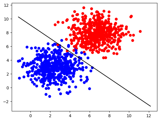
3 - Performance on a Larger Dataset#
Construct a larger and more complex dataset with the function make_blobs from the sklearn.datasets library:
# Dataset
n_samples = 1000
samples, labels = make_blobs(n_samples=n_samples,
                             centers=([2.5, 3], [6.7, 7.9]),
                             cluster_std=1.4,
                             random_state=0)

X_larger = np.transpose(samples)
Y_larger = labels.reshape((1,n_samples))

plt.scatter(X_larger[0, :], X_larger[1, :], c=Y_larger, cmap=colors.ListedColormap(['blue', 'red']));
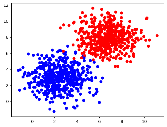
And train your neural network for \(600\) iterations.
parameters_larger = nn_model(X_larger, Y_larger, num_iterations=600, learning_rate=0.1, print_cost=True)
print("W = " + str(parameters_larger["W"]))
print("b = " + str(parameters_larger["b"]))
Plot the decision boundary:
plot_decision_boundary(X_larger, Y_larger, parameters_larger)